

Since FIFA decreed these rules upon the footballing globe, all of football’s transfer business has been squeezed into these two windows. During the twelve weeks of last summer’s transfer window, the 20 clubs in the English Premier League alone spent over £835m!
Despite these huge sums of money, analysts in the media judge player acquisitions based on just a few of the most basic of statistics: goals scored and pass completion percentage being two of the more popular ones. With regards to clubs themselves, whatever statistical analysis they use for player recruitment is kept secret. However, we suspect some owners and managers buy (and sell) players largely on gut instinct, along with these most basic statistics.
This lack of statistical analysis is not seen in all sports. In the US, sports have embraced statistics in aiding player recruitment and playing strategy. Of course, baseball pioneered the use of statistics – the story of how the Oakland Athletics competed at the very highest level on just a fraction of the budget of the other top teams has rapidly become stats folklore.
In football, progress is slow at best. In part this is a consequence of the nature of the game. Football is very dynamic with many players interacting continuously during each game. This is not a simple setting for a statistician to say the least. But technological advances have meant the dynamic nature can now be recorded pretty well.
Some public attempts have been made to rate players, like EA Sports PPI or the Castrol Index. But these indices measure past performance and attempt to answer the question: ‘Who is the best player of this current season’. When buying players this isn’t quite what you want – you need to make decisions on who to buy based on predicted future performance, not observed past performance. We wanted to see if we could model this future performance.
To do this we obtained data1 on all matches in the English Premier League for the two seasons, 2006-07 and 2007-08. For our purposes (identifying goal scoring ability) we are interested in shot events only, leaving us with 804 goals from 7,678 shots in our fitting sample (the first season). Our aim was to try to predict future performance on what is arguably the most important single statistic in football – goals.
Why can’t we just use goals, or goals per minute played?
Football is not a perfect experiment, and simple statistics like goals scored, or goals per minute played are biased as a consequence of players playing for and against teams of different quality. Furthermore, no two players can be expected to play the same number of minutes or take the same number of shots. For example, if one player scored 3 goals in 4 matches whilst another player scored 8 goals in 16 matches – who would you buy?
To deal with these problems, we adopted a mixed effects model to identify the goal scoring ability of players.
A model for scoring goals
To model the goal scoring process, we break it down into two constituent components: the process of generating shots and the process of converting shots to goals. This specification means we can measure how shot creation and shot conversion depend on, for example, the player’s team, the opposition, and the player’s own ability as well as chance2 (see footnotes).
The model gives two types of predictions:
- Complete predictions that assume knowledge of everything during every game e.g. time on the pitch and identity of the opposition etc.
- Averaged predictions that effectively assume all players play for the same amount of time, for the same side, against all other teams. For these predictions there are no biases resulting from players playing for top teams and players can be compared on a level field.
We are only going to present the results of the averaged predictions as these are what are useful when comparing players in the transfer market.
So what should a club look for in a goal scorer?
‘A plot says a thousand words’, probably more so in statistics. The plot below (figure 1) summarises the shot count model.
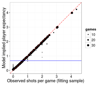
Figure 1: Shot generation: average model implied predictions versus the average observed values per player in the fitting sample.
The dashed line is the identity function. The horizontal line is the average number of shots per game. Each dot is a player and the size of the dot indicates the number of games played in the fitting sample.
There is some evidence of regression to the mean, in that observed high shot counts (the x-axis), are dragged back towards the horizontal line and low shots counts are pushed up towards the horizontal line. The effect is bigger for smaller dots. This represents the fact that our uncertainty about a player’s shots-per-game is higher for players who play in very few games.
For the shots to goals conversion model, shown in the next plot (figure 2) below, the regression to the mean is much stronger. A very high rate of conversion is regressed right down towards the mean for the previous year and vice versa for low conversion rates. It is remarkable that the observed range lies between 0 and 100% whilst the predicted range lies between 7% and 17%.
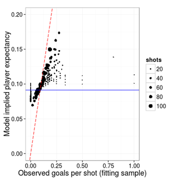
Figure 2: Shot conversion: average model implied predictions versus the average observed values per player in the fitting sample.
The table below gives the results for the 2006/07 season. Didier Drogba of Chelsea was identified as the player with the highest goal scoring ability, with Ronaldo in second place. In general, you can see how the model regresses the performance of the top players towards the mean and this appears to be the right thing to do as the model predictions are closer to the observed 2007/08 goals per 100 minutes for 10 out of the 15 players.
| Predicted and actual 2007/2008 goals per 100 minutes for the top 15 players. Model predicted goals per 100 minutes scorers based on season 2006/2007 data. | ||||||
| Rank | Player | 2006/2007 | 2007/2008 | Model | Naïve | Actual |
| 1 | Drogba | Chelsea | Chelsea | 0.47 | 0.62 | 0.54 |
| 2 | Ronaldo | Man Utd | Man Utd | 0.42 | 0.46 | 0.97 |
| 3 | Van Persie | Arsenal | Arsenal | 0.39 | 0.66 | 0.20 |
| 4 | Rooney | Man Utd | Man Utd | 0.36 | 0.40 | 0.57 |
| 5 | Viduka | Middlesbrough | Newcastle | 0.36 | 0.66 | 0.38 |
| 6 | Crouch | Liverpool | Liverpool | 0.36 | 0.51 | 0.37 |
| 7 | Vaughan | Everton | Everton | 0.32 | 0.58 | 0.00 |
| 8 | Berbatov | Tottenham | Tottenham | 0.32 | 0.43 | 0.51 |
| 9 | Kuyt | Liverpool | Liverpool | 0.31 | 0.45 | 0.05 |
| 10 | Defoe | Tottenham | Tottenham / Portsmouth | 0.31 | 0.35 | 0.65 |
| 11 | Saha | Man Utd | Man Utd | 0.29 | 0.30 | 0.18 |
| 12 | Cole | Portsmouth | Sunderland | 0.28 | 0.41 | 0.00 |
| 13 | McCarthy | Blackburn | Blackburn | 0.28 | 0.44 | 0.19 |
| 14 | Zamora | West Ham | West Ham | 0.27 | 0.41 | 0.00 |
| 15 | Adebayor | Arsenal | Arsenal | 0.27 | 0.34 | 0.62 |
The final plots (figure 3) nicely summarise the performance of the averaged predictions. Keep an eye on the plot on the left which can be thought of as the predicted goals per 100 minutes on the x-axis with the observed goals per 100 minutes on the y-axis (we are using the 2006-07 data as the prediction for 2007-08).
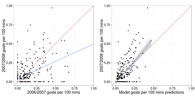
Figure 3: Goals per 100 minutes played for 2007/08 versus goals per 100 minutes played for 2006/07 (left) and versus model predictions (right).
The relationship between the model predictions and the observed 2007-08 goals per 100 minutes, shown by the blue line (which is a linear regression fit plus a 95% confidence interval) is much stronger. In fact, the bias observed in the plot on the left has been over-corrected for.
It turns out that this over-correction is not flaw in the model, rather it is a consequence of using the averaged predictions rather than complete predictions. For example, the model under predicts the goals by the very top players because they are more likely to play for the very top teams. As such, on average, they will actually be facing weaker teams than the averaged predictions presume. The equivalent plot for the complete predictions lies almost perfectly on the dashed line.
A player’s record of generating shots is more important than their record of converting shots to goals
In this work, we have concentrated on just one aspect of a footballer’s set of skills – goals. There are of course many other skills required of a footballer. Still, our mixed effects model for goals has proved to be an improvement on simple count-type statistics currently used to rate goals scorers. Just in case the chief executive of a football club is reading Significance, a key finding of our work is this. Generating shots is more predictable than converting shots.
Of course, a chief executive could just use our model which accounts for both aspects of performance in identifying goal scoring ability! If you are spending several £100m on players in the next transfer window, you could do worse that to speak to a statistician before handing over your money.
Footnotes
1. Opta provides an incredibly rich data set describing football statistics. Data are available on the position (x-y coordinates), timing (seconds), players involved, and event type (pass, tackle, goal, foul and many more) for every event that happens during a football match. This is incredibly granular data. A typical match consists of several thousand rows of events.
2. Let n be the number of shots and y be the number of goals. We model the distribution of goals:
\begin{equation}
p(y)= \sum_n p(y|n)p(n).
\end{equation}
This gives us two models to fit: one for shot generation and one for goals given the number of shots.
For the shot count model, we assume that $n \sim Poisson(e^{\eta})$ and we let $\eta$ be a linear function of some covariates. Namely, player identity, home advantage, own team strength and opposition strength. Most importantly, we assume the players’ abilities to create shots are random and normally distributed, so that they are random effects but in this model we are very much interested in the values of each random effect which represent the player’s ability to generate shots.
For the shots to goals conversion model we assume that $y|n \sim binomial$ with linear predictor equal to a linear function of the covariates as used in the shot generation model. This time, we assume the players’ abilities to convert shots to goals are random effects which are normally distributed.


