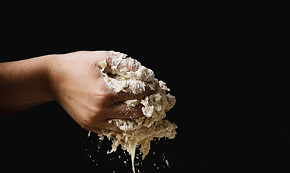

Letisha Smith – winner of the 2018 Award for Statistical Excellence in Early-Career Writing – started the year with the resolve to eat smarter, with less food and less money going to waste. She turned to machine learning to help streamline her meal plans.
EDITOR’S NOTE Letisha Smith’s award-winning article was originally published in the October 2018 issue of Significance. We are republishing her article online as we prepare to launch our 2019 writing competition. Details of this year’s contest will be published here in early February. In the meantime, check out the full list of published articles from past winners and finalists.
As the New Year commenced, I resolved – along with many other Americans – to adopt healthier eating habits. But after checking out a few fad diets and nutrition guidelines, I noticed a common flaw in most meal plans. Daily menus have their own set of ingredients that are rarely reused. It’s as if each meal was planned in a silo, without much consideration of ingredients left over from other dishes.
If one chose to follow most meal guides, dietary goals would be met at the expense of a refrigerator full of unused ingredients – most of which would likely end up in the garbage. Indeed, it is estimated that one-third of food produced for human consumption is trashed before reaching our plates.
Food waste can be reduced at the consumer level through planning multiple meals that share similar ingredients, and this has traditionally been achieved by finding recipes that use leftover ingredients. However, this approach is reactive, not proactive. I wondered: is there an easier way to find recipes that share ingredients without pre-specifying the leftovers? Could machine learning be used to maximise the number of meals made with a minimal amount of ingredients?
Recipe for success
Data analysis is like the human diet: if you put garbage in, you get garbage out. So before identifying recipes with similar ingredients, I needed to ensure that the recipes I selected were of good quality. My first step was to consult Allrecipes.com, which ranks as the internet’s most popular recipe site, according to internet research firm Alexa. Unlike other sites where recipes are curated by editors and celebrity chefs, the content on Allrecipes.com is generated and reviewed by its users.
As of May 2018, the site’s main meals section contained over 14 000 recipes. I extracted these recipes using the rvest package in R, which makes it easy to download and manipulate HTML and XML content. Main meals, on average, had 92 reviews and scored 4 out of 5 stars, so to narrow my selection to the very best-rated recipes, I analysed only those with a mean of at least 4.5 stars. Furthermore, to ensure that scores were stable, the final data set included only recipes with at least 132 reviews, a criterion met by the top 15% of dishes. These qualifications narrowed the analysis to 909 recipes.
Text prep: slicing and dicing
Weaning toddlers quickly learn that food must be chewed before it is swallowed. Similarly, my list of ingredients from each recipe needed to be “byte sized” before algorithmic digestion. For computers, simple text comprehension ignores tone or syntax, and translation occurs through calculation. Words in a text document are tallied, and topics can be deciphered by word frequency. Summarizing by word counts easily communicates the topic of a text when the following are removed:
- punctuation and numbers;
- stop words – such as “be”, “can”, and “the” – that are commonly used in communication regardless of context; and
- suffixes – “-ed”, “-ing”, and “-es” – so that words sharing the same root appear identical.
This approach treats text as a bag of words, and it works well with narrative text. However, recipes are instructional and require a tweaking of the above steps for best results.
As humans, it is easy to look at recipe ingredients presented as either “1 ear corn on the cob, unhusked” or “2 eight-ounce bags of frozen corn” and know that the food to buy is corn. All the other words can therefore be categorized as stop words that should be removed. However, with over 900 recipes, sifting through ingredients to build a list of words to remove would be too time-consuming at best. At worst, subjectively editing the data could bias the analysis.
Therefore, after careful consideration, I changed my approach from eliminating superfluous text to retaining words representative of foods. All I needed was a list of food words to compare to recipe ingredients. Then a spreadsheet could be created where each row represented a recipe, and each column was a distinct food from the food list. If a food from the list was found in a recipe, a 1 would populate under the respective food column. Zeros would be placed in columns where the food was not a recipe ingredient. With this approach, detecting foods and removing non-essential words could seamlessly occur in one step.
Fortunately, I gained access to a proprietary list containing several thousand food words, which made it easy to extract the key information from each list of ingredients. The food list was comprehensive and contained not only different spellings of words like “lasagna” and “lasagne”, but also proper nouns like “Golden Delicious apple” and “Granny Smith apple”. Having columns for general and proper nouns is useful because if a recipe specifically uses a “Gala apple” then a 1 goes in the “Gala apple” column in addition to the general apple column. The 1s under each column make it easier to identify recipes that share general and specific ingredients.
Approximately 600 words from the food list were found among the recipe ingredients. Therefore, I had a spreadsheet (or data matrix) with over 900 rows for the recipes and about 600 columns representing the foods extracted from the ingredients. With the text prep complete, it was time to consider the best way to group together recipes.
A smidgen of similarity
When it comes to categorising foods, the best organisation systems designate distinct groups that share common characteristics. Furthermore, each group should be unique and contain foods with a set of commonalities that are different enough from other groups to justify annexation.
These criteria lead one to ponder the best way to measure a group’s internal similarity and external uniqueness. Similarity and uniqueness both describe how close items are to one another, which suggests that the general distance formula of valueobject2 – valueobject1 could be used to quantify ingredient differences in recipes. In this analysis, recipes are the objects being measured for similarity, and the values come from the 1s and 0s placed in each food column.
For example, let us use values in the tomato column to quantify how similar two recipes are. If two recipes both use tomatoes, then they will both have 1s under the tomato column, and 1 – 1 = 0, which supports the conclusion that the recipes are alike on this food dimension.
Furthermore, if neither recipe contains tomatoes, then they will both have 0s under the tomato column and the two recipes still have zero difference on this food dimension.
However, if the second recipe contains tomatoes and the first one does not, then the recipes will respectively contain a 1 and 0 in the tomato column: 1 – 0 = 1, which demonstrates that the recipes are different on this food dimension.
The distance formula is the foundation for some of the most common measures of proximity. Variations like Euclidean and Manhattan distance respectively transform the difference to always be positive by squaring the result or taking the absolute value. For example, if the first recipe contains tomatoes and the second one does not, then 0 – 1 = –1, which is negative. However, the difference becomes positive once it is squared or made absolute.
The calculations above were for a single food dimension, but each recipe had values from over 600 food dimensions, which could be used to calculate ingredient differences. After measuring the distance between two recipes on all dimensions, the sum of the differences can be taken to represent how similar all the ingredients in one recipe are to another. Lower totals suggest that recipes share common ingredients, and higher totals suggest that recipe ingredients are different.
For quantifying ingredient similarity, I found the Manhattan approach for distance calculations most effective. When an object has data for hundreds of dimensions, it is common for the data to have many zeros, indicating that the object does not have a value for that dimension. Most recipes have about 10 ingredients, so for any given recipe, a majority of columns contain zeros to represent the absence of a food. For some distance metrics, too many zeros make it challenging to detect similarities beyond having zeros for the same dimension. This problem is known as the curse of dimensionality, and it can be attenuated by using Manhattan distance, which accommodates high-dimensional data well. Manhattan distance essentially sums the absolute differences of all dimensions.1
Once the sum of differences is calculated for all recipe pairs, then values can be sorted to indicate recipes that are most and least similar to one another. Having a way to measure and compare recipe pairs by ingredient composition left me one step away from accomplishing the goal of identifying groups of recipes with shared ingredients.
Dinner deconstructed
With over 400 000 similarity values for each unique pair of recipes, I desired a more palatable presentation of the data. I knew that recipes from the same cuisine often use similar ingredients, but beyond that I had no clue as to how many specific groups were encompassed under the broader main meals category. I thought it made sense to start the first group by joining the two most similar recipes together, yet was uncertain how to proceed from there.
Fortunately, dendrograms are a powerful approach to visualising the distance between items and elucidating an unknown number of groups from a collection. Dendrograms (Figure 1) are a graphical representation of hierarchical clustering, which starts by placing each item in a group by itself. All one-item groups are represented by minuscule dots at the bottom of the dendrogram. Then the two most similar items are merged to form the first pairing. Merges are represented by each dot being connected by upward lines, with heights proportional to the level of similarity.2
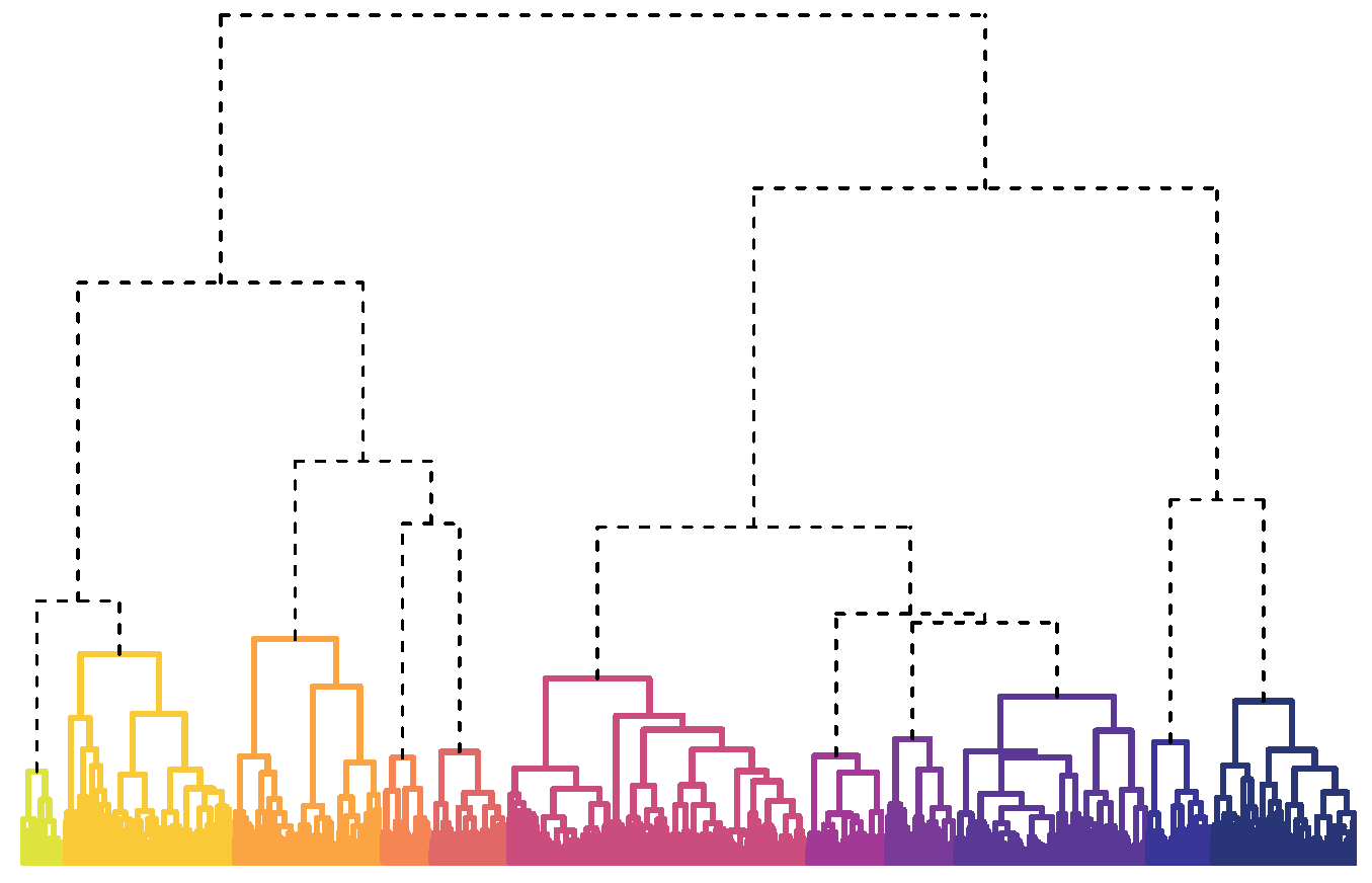
FIGURE 1 Dendrogram of 11 recipe groups. Names of coloured groups are given in Table 1.
TABLE 1 Details of each recipe group, including total number of recipes within each group, ingredients and example recipes. The final column reports the expected percentage of shared ingredients when selecting recipes at random within each group.
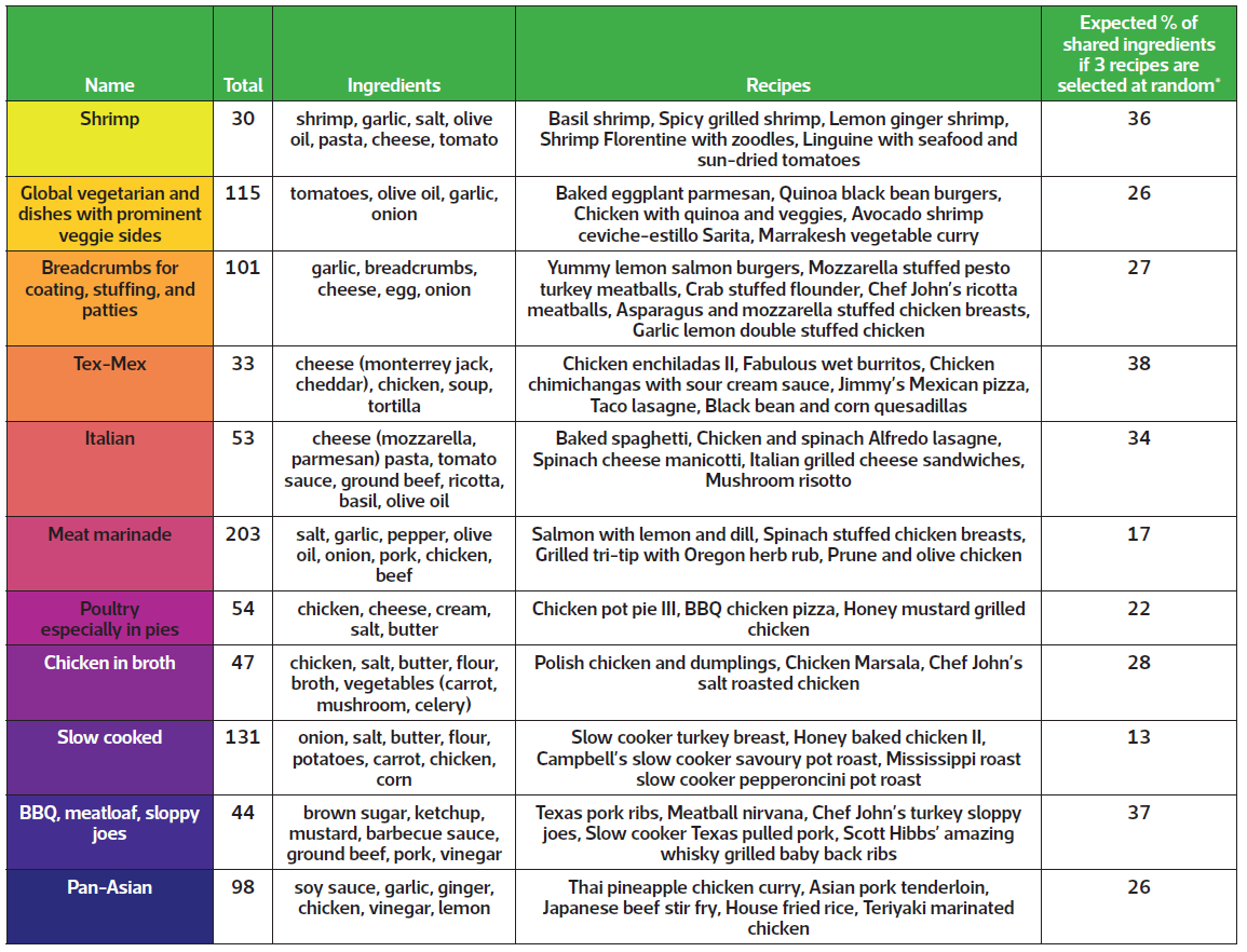
* Values were estimated by drawing 10 000 samples from each group.
After the first join, distances between the paired group and all other one-item groups must be determined. For example, let us assume that a lasagne and spaghetti recipe are the most similar dishes because they both require noodles, tomato sauce, basil, and parmesan cheese, so these recipes are consolidated first. However, there is also a pizza recipe made with dough, tomato sauce, parmesan cheese, and mozzarella cheese. Therefore, there is a need to evaluate if the next join should be adding pizza to this pasta group.
Because lasagne uses mozzarella and spaghetti does not, the difference between lasagne and pizza is not identical to the distance between spaghetti and pizza. So, one must decide how to aggregate the individual differences between the pizza and each pasta dish to represent the total distance between cheese pizza and the pasta group.
Hierarchical clustering uses agglomerative methods to address the measurement of space between groups. The single linkage approach suggests that the space between pizza and the pasta group be represented by the distance between pizza and lasagne because this value is smaller. Meanwhile, the complete linkage approach suggests using the distance between pizza and spaghetti because it is larger.
The choice of agglomeration method is complex and often dependent on relationships within the data. I received the best agglomeration results by implementing Ward’s method, which aims to produce groups with high internal homogeneity. I desired groups of recipes that contained common ingredients, so it was important for the grouping algorithm to maximize similarities.3
Groups are considered to be most homogeneous when they initially contain a single item or recipe. Consequentially, as group size increases so group diversity increases. Quantifying how the diversity of a paired group increases with an additional item can be generally calculated by measuring variationbetween groups – variationwithin group.
“Within group” variation is the similarity value previously calculated. Therefore, variation within the pasta group is the measurement of similarity between lasagne and spaghetti.
“Between group” variation is the total similarity between the single-item group and each item in the paired group. For the pasta and cheese pizza groups, between group variation is essentially the sum of the similarity scores for pizza and spaghetti, and pizza and lasagne. Ultimately, pizza would only be added to the pasta group if it were the dish most similar to the pastas, and no other pair of more similar recipes needed to be joined first.
Hierarchical clustering is complete once all items have been incrementally joined to form a single collection. Because all items are ultimately united, hierarchical clustering lacks precise group divisions. Dendrograms suggest group divisions when longer lines are used to connect clusters. However, a more empirical approach to selecting the best number of groups is to use one of many indices developed to identify divisions that produce groups with minimal internal diversity and considerable external differences.
I used many popular indices to evaluate the best number of divisions, and results consistently suggested that the data was best divided into two groups. However, each group contained too many recipes with broad ingredient combinations. Therefore, it was difficult to identify foods that commonly recurred in either set of recipes.
Instead, I explored other divisions and determined that the data could be meaningfully partitioned into 11 groups that are presented in Figure 1 and Table 1. Categories mostly represent cuisines, such as Italian and Tex-Mex, or proteins, like chicken and shrimp, which feature prominently in the US diet. Some foods, like cheese, tomatoes, onions, and olive oil, are common between groups and desirable for making a variety of meals.
The analysis serves as a proof of concept that recipes with shared ingredients can be grouped before pre-specifying ingredient combinations. If someone were to select at random three of the recipes included in the analysis, then – on average – about 15% of the ingredients would be used in more than one recipe. However, if one were to select at random three recipes from groups like the Tex-Mex or barbeque categories, then 30–40% of the required ingredients would be expected to be used in more than one dish. Selecting meals from the same category therefore enables one to use the same ingredients in multiple dishes without too much up-front planning – potentially reducing food waste in the process.
Acknowledgements
I would like to thank Yoav Bergner, Marc Scott, and Maxwell Austensen of New York University for their supportive advice while working on this project.
About the author
Letisha Smith is an Atlanta, Georgia native, who recently graduated with a master’s in applied statistics from New York University. She currently works at the Institute for Innovations in Medical Education, which is a part of NYU’s School of Medicine.
References
- Aggarwal, C. C., Hinneburg, A. and Keim, D. A. (2001). On the surprising behavior of distance metrics in high dimensional space. In J. Van den Bussche and V. Vianu (eds), Database Theory – ICDT 2001 (pp. 420–434). Berlin: Springer. ^
- Greenacre, M. and Primicerio, R. (2014). Multivariate Analysis of Ecological Data. Bilbao: Fundación BBVA. ^
- Strauss, T. and von Maltitz, M. J. (2017). Generalising Ward’s method for use with Manhattan distances. PloS ONE, 12(1), e0168288. ^


